Agentic Phi4 Summary - Logarithmic Regressions

research_foundational

---

Logarithmic Regression Overview

Introduction

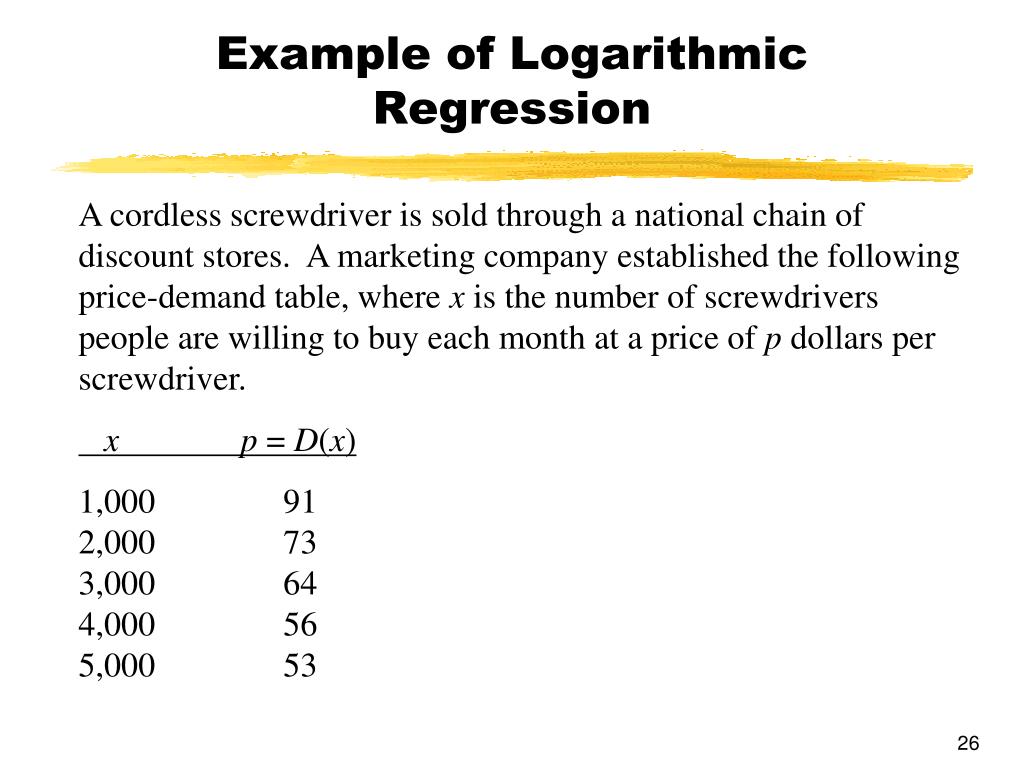
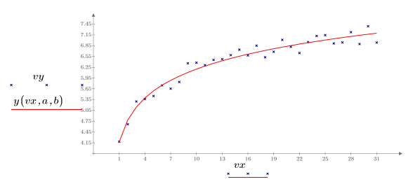
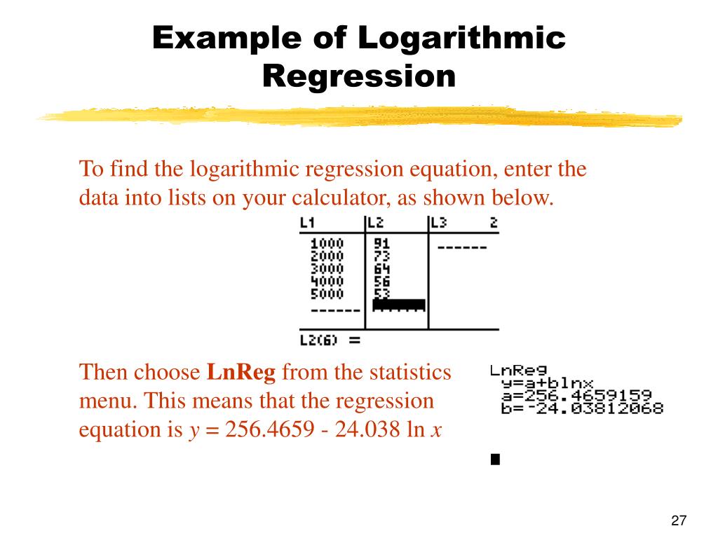
Logarithmic regression is a statistical technique used to model situations where growth or decay initially happens rapidly and then slows over time. It applies a logarithmic function to the data, typically expressed in the form ( y = a + b \ln(x) ). This method is especially useful when there’s a significant variation in the rate of change across the range of the independent variable.

Application

• Growth/Decay Modeling: Commonly used in scenarios where changes are not linear but instead exhibit rapid initial growth or decay that tapers off.
• Predictive Analysis: Helps predict ( y )-values either within the observed data range (interpolation) or beyond it (extrapolation).

Tools and Calculations

Various tools can perform logarithmic regression, providing outputs such as:

• Regression equation
• Correlation coefficient (( r ))
• R-squared value (( r^2 ))

These calculations help assess how well the model fits the data.

Considerations

While dimensionally valid data can always undergo logarithmic regression, it’s important to evaluate the quality of fit. The suitability and accuracy of a logarithmic model depend on the nature of the data being analyzed.

By understanding these components, one can effectively apply logarithmic regression in statistical analysis to draw meaningful insights from data exhibiting non-linear growth or decay patterns.

code_snippets

---

Below are some examples demonstrating how to perform logarithmic regression in Python using the numpy and scipy libraries. These examples will help a junior engineer understand both the concept and implementation of logarithmic regression.

Basic Logarithmic Regression

Purpose: Perform a basic logarithmic regression on sample data points, fitting the model ( y = a + b \ln(x) ).

import numpy as np
from scipy.optimize import curve_fit
import matplotlib.pyplot as plt
 
# Sample data: predictor and response variables
x_data = np.array([1, 2, 3, 4, 5])
y_data = np.array([0.5, 1.3, 2.1, 3.6, 4.8])
 
# Logarithmic function to fit the data
def log_func(x, a, b):
    return a + b * np.log(x)
 
# Fit the model to the data
params, covariance = curve_fit(log_func, x_data, y_data)
a, b = params
 
# Plot original data and the fitted logarithmic line
plt.scatter(x_data, y_data, label='Data')
plt.plot(x_data, log_func(x_data, a, b), label=f'Fit: y = {a:.2f} + {b:.2f}*ln(x)', color='red')
plt.xlabel('x')
plt.ylabel('y')
plt.legend()
plt.show()
 
print(f"Fitted parameters: a = {a:.2f}, b = {b:.2f}")

Calculating Correlation and R-squared

Purpose: Calculate correlation coefficient ((r)) and R-squared value to evaluate the fit of the logarithmic regression model.

# Predicted values using the fitted model
y_pred = log_func(x_data, a, b)
 
# Calculate the correlation coefficient (r) and R-squared (R^2)
correlation_matrix = np.corrcoef(y_data, y_pred)
r = correlation_matrix[0, 1]
 
ss_res = np.sum((y_data - y_pred)**2)
ss_tot = np.sum((y_data - np.mean(y_data))**2)
r_squared = 1 - (ss_res / ss_tot)
 
print(f"Correlation coefficient (r): {r:.2f}")
print(f"R-squared (R^2): {r_squared:.2f}")

Example with More Data Points

Purpose: Demonstrate the effect of more data points on logarithmic regression fitting.

# Additional data for a better fit demonstration
x_data = np.array([1, 2, 3, 4, 5, 6, 7, 8, 9, 10])
y_data = np.array([0.7, 1.4, 1.9, 3.4, 4.9, 6.2, 7.8, 8.1, 9.5, 11.0])
 
# Fit the model to the extended data
params, covariance = curve_fit(log_func, x_data, y_data)
a, b = params
 
# Plot and show results
plt.scatter(x_data, y_data, label='Data')
plt.plot(x_data, log_func(x_data, a, b), label=f'Fit: y = {a:.2f} + {b:.2f}*ln(x)', color='green')
plt.xlabel('x')
plt.ylabel('y')
plt.legend()
plt.show()
 
print(f"Fitted parameters with more data: a = {a:.2f}, b = {b:.2f}")

These examples illustrate how to fit and evaluate logarithmic regression models in Python, helping you understand the underlying mechanics and statistical measures associated with these models.

cite_sources

---

Citations for Logarithmic Regressions

1. Statology. (n.d.). Logarithmic Regression in Python (Step-by-Step).
2. MathBitsNotebook. (n.d.). Logarithmic Regression (LnReg).
3. LibreTexts. (n.d.). 6.9: Exponential and Logarithmic Regressions.](https://math.libretexts.org/Workbench/1250_Draft_3/06:_Exponential_and_Logarithmic_Functions/6.09:_Exponential_and_Logarithmic_Regressions)
4. Statology. (n.d.). Logarithmic Regression Calculator.
5. ZScoreCalculator. (n.d.). Logarithmic Regression Calculator.
6. MathCracker.com. (n.d.). Logarithmic Regression.
7. Statology. (n.d.). How to Perform Logarithmic Regression on a TI-84 Calculator.
8. Outlier. (n.d.). Calculating Logarithmic Regression Step-by-Step.
9. Statology. (n.d.). Logarithmic Regression in Excel (Step-by-Step).

Embedded Images

1. 
2. 
3. 
4. 
5. 

These citations and resources provide a comprehensive overview of logarithmic regressions, suitable for those using Obsidian.md.